Tutorial

Introduction

c2raytools can be used in two ways: either interactively from a Python prompt, or as part of a Python script. Here, we will show how to use it interactively, but the code is of course the same if you use it from a script.

Reading files

The most common thing you will want to do is to read data files. c2raytools contains a number of classes for reading xfrac, density, velocity and halo list files.

Say you want to read the ionized fraction and density data at some redshift. First, start up your favorite Python interpreter, for example IPython, and import c2raytools:

>>> import c2raytools as c2t

The first thing you want to do is to set the conversion factors. Since much of the data is stored in physically meaningless simulation units which vary between different simulation runs, c2raytools needs to know how to convert these to physical units. To do this, there is a function called set_sim_constants(). This function takes as its only parameter the box side in cMpc/h. To specify that you are using the 114/h cMpc simulation, run:

>>> c2t.set_sim_constants(114)

If this function is not run, the default box size is 114/h cMpc (so in this case, we could in fact have skipped this step, but it’s a good habit to always run this function).

Sometimes, it is useful to get feedback on what is happening. If you wish, you can turn on verbose mode by running:

>>> c2t.set_verbose(True)

Now, we can load our ionization fraction file:

>>> my_x_file = c2t.XfracFile('/path/to/datafiles/xfrac3d_8.515.bin')

and the density file:

>>> my_d_file = c2t.DensityFile('/path/to/datafiles/8.515n_all.dat')

The objects my_x_file and my_d_file now hold the data from the files. You can access the ionization fraction and density as the numpy arrays xi and cgs_density. Since these are numpy arrays, you can of course perform all of numpy’s indexing and slicing methods, and calculate simple statistics. For example, here we are printing the ionized fraction in cell (0,10,100) and calculating the mean density in g/cm^3:

>>> my_x_file.xi[0,10,100]
0.0305728369737
>>> my_d_file.cgs_density.mean()
4.04777106867e-31

For the full documentation on the file reading routines, see File classes.

Other file formats

There are also a methods to read and save data from files in a number of other file formats that are commonly used for data derived from C2-Ray output. For example, you can read and save files in cbin format (raw binary with three inital integers specifying the mesh size):

>>> data = c2t.read_cbin('myfile.cbin')
>>> c2t.save_cbin('myotherfile_64bit.cbin', data, bits=64)

You can also read and save files in fits format:

>>> c2t.save_fits(data, 'myfile.fits')

Visualizing data

You can of course plot the data you read using your favorite plotting software. For example, if you have matplotlib installed, you can plot a slice through a density cube:

>>> import pylab as pl
>>> pl.imshow(my_d_file.cgs_density[0,:,:])
>>> pl.colorbar()

However, there are also a couple of convenience methods in c2raytools that make the most common plotting tasks easy. One such task is to plot a slice through a data cube. This can be done easily using the function plot_slice():

>>> c2t.plot_slice(my_x_file)

This will produce an image that looks something like this:

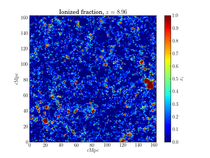
You can give plot_slice() objects of type XfracFile or DensityFile or a string with the name of a file, and it will figure out what to do with the data. By default, it plots a slice along the first coordinate axis, at a coordinate value of zero. This can be changed with the arguments los_axis and slice_num.

In this example, plot_slice() will automatically read a density file and plot a slice at y = 10:

>>> filename = '/path/to/data/8.515n_all.dat'
>>> c2t.plot_slice(filename, los_axis = 1, slice_num = 10)

There is also a function called plot_hist(). This function works similarly to plot_slice(), but instead plots a histogram of all the values in the data cube. This example reads an xfrac file and plots a histogram of the ionized state of all the cells:

>>> c2t.plot_hist('/path/to/datafiles/xfrac3d_8.515.bin')

See Visualizing data for the full documentation.

Analyzing files

In addition to the file reading routines described above, c2raytools includes many functions to perform common operations and calculate statistics from the data, as well as some cosmology functions. For example, you can calculate the differential brightness temperature from a density file and an xfrac file:

>>> dT = c2t.calc_dt(my_x_file, my_d_file)

There are also a number of routines for calculating power spectra. For example, to calculate and plot the spherically averaged power spectrum of the ionized fraction, you can run:

>>> ps, k = c2t.power_spectrum_1d(my_x_file.xi)
>>> pl.loglog(k, ps)
>>> pl.xlabel('$k \; (Mpc^{-1}$')
>>> pl.ylabel('$P(k) \; (Mpc^3)$')

You can also convert data from real space to redshift space:

>>> dfile = c2t.DensityFile('/path/to/data/8.515n_all.dat')
>>> vfile = c2t.VelocityFile('/path/to/data/8.515v_all.dat')
>>> kms = vfile.get_kms_from_density(dfile)
>>> distorted = c2t.get_distorted_dt(dfile.raw_density.astype('float64'), kms, dfile.z, los_axis=0, num_particles=20)

For more examples on what you can do, and full documentation on the various functions, see the full Documentation, or browse through the index. Also have a look at the example scripts included with the module.