Radiative cooling

Astrophysical gases tend to radiate when heated. This radiation is an energy leak which may carry away substantial amounts of energy. A simulation which does not include the radiative cooling (such as the one in the previous section) is often referred to as an adiabatic simulation.

Figure 3: The coronal cooling curve from Dalgarno & McCray (1972)

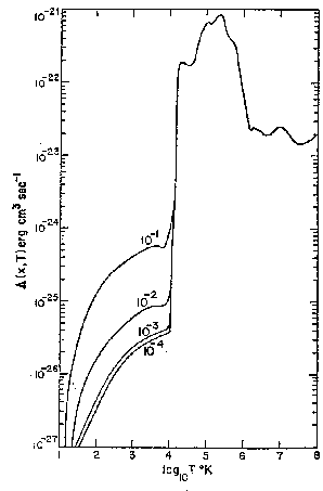
The file corocool.tab (in anonymous ftp) contains what is called a coronal cooling curve. The file contains two columns, the first one lists the log of the temperature, the second one the log of the cooling $\Lambda$ in units of erg cm$^3$ s$^{-1}$. This particular cooling curve is taken from Dalgarno & McCray (1972), reproduced here as Fig. 3. It was calculated by determining the equilibrium ionization state at every temperature and from that the amount of emission. Below $10^4$ K the cooling depends strongly on the ionization fraction of the gas, the one in the table is the curve labelled $10^{-4}$ in the paper. The cooling rate of a gas can be approximated by $n^2 \Lambda(T)$, where $n$ is the number density of particles.

Numerically, the cooling is a source term for the energy density and can be included in a similar way as the geometric source terms, i.e. in a separate calculation every time step. However, there is the danger that the cooling will reduce the temperature/internal energy density below zero, which is unphysical. The reason for this is the very non-linear behaviour of the cooling function. There are two ways to control this:

• Limit the time step not only with the CFL condition, but also with the cooling time. Limit the change of internal energy to something like 10% per time step. This may lead to very short time steps, perhaps too short in be practical (experiment with this).
• Solve the equation implicitly, i.e. find the new energy density or temperature and use this to find a new and better estimate for the change in energy density. Implicit methods are described in any book on numerical methods, for example in Numerical Recipes.

The best solution for situations in which heating is solely by shocks (as we have here) is to try to resolve the so-called cooling region. In a shock the temperature is first raised to the post-shock value and then as it moves away from the shock it cools. If this cooling region is contained in one cell of your calculation you are not resolving this process and the solution will be some average temperature and density which could have little to do with the real average density and temperature in the cooling region. In this case you will also have to use extremely short time steps or an implicit solution. If however the cell size is small enough to follow the post-shock cooling you will not only have a more accurate representation of the post-shock region, but also much less problems with solving for the cooling, since the change in internal energy density will be small per time step. For safety reasons one can still limit the time step with the cooling time, but usually the cooling time will be of order of or less than the CFL time.

A) Solve the problem from Section 2 with radiative cooling included. Still assume that all material is ionized. What differences are there with the non-cooling solution? Why is the effect larger for the outer shock than for the inner shock? Is it possible to resolve the cooling region? What compression (density jump) do you find for the swept up shell?

If you are unsuccessful in getting the code to run with cooling, you can try lowering the overall density. This will reduce the cooling rate. You could for instance try $\dot{M}=10^{-8}$ $M_\odot$ yr$^{-1}$ and $\dot{M}=10^{-6}$ $M_\odot$ yr$^{-1}$ for the fast and slow wind respectively. A 10 times lower density gives a 100 times lower cooling. If you reduce the density too much the result of the calculation will be the similar to the one without cooling.

B) Follow the interaction between a moderately fast wind and an outer slow wind. Use the following parameters: $\dot{M}=10^{-7}$ $M_\odot$ yr$^{-1}$, $v=120$ km s$^{-1}$ for the fast wind, and $\dot{M}=10^{-6}$ $M_\odot$ yr$^{-1}$, $v=10$ km s$^{-1}$ for the slow wind. First do a simulation without cooling and then add the cooling. Compare the two results and also compare them to the differences between the non-cooling and cooling simulation for the 1000 km s$^{-1}$ wind. Why is the behaviour of the inner shock very different?

C) A weakly cooling bubble is often called energy conserving and a strongly cooling bubble momentum conserving. Lamers & Cassinelli (1999) state in Sect. 12.3 of their book that one can observationally check whether a bubble is momentum or energy conserving by considering the following ratios:

$\epsilon$=(total kinetic energy in shell)/(total wind energy provided)

$\pi$=(momentum in the shell)/(momentum imparted by the wind)

If $\epsilon\approx 1$ the shell is energy conserving, whereas when $\pi\approx 1$ it is momentum conserving.

Check whether the shells in your models are indeed energy conserving and momentum conserving according to these definitions, by calculating $\epsilon$ and $\pi$ for both cases.