
Axel Runnholm
PhD Student in Astronomy
Stockholm University
axel.runnholm [at] astro.su.se
08-5537 8502
Projects
Lyman Alpha Reference Sample
A sample of local starbursting galaxies which is used to understand the complex physics of Lyman alpha transfer and escape.Galaxy Wind Synthesis
This is a project where we are trying to understand the connection between stars and galaxy scale outflows.Research notes / blog
Principal Component Analysis
10-01-2018
Research Notes And Blög
Here I have collected some notes and texts primarily for my own use, but published online in order to force some effort to be made concerning the format of the text.Principal Component Analysis
10-01-2018
What does it do?
In a nutshell principal component analysis find the directions that contain most of the information in a dataset. Basically it uses a matrix analysis to find whatever direction in the dataset contains the largest spread, variance, in the data and uses this as the first basis vector, or axis, of a new coordinate system. Then the next axis is chosen along the direction of the second largest variance but constrained to be orthogonal to the first axis. This procedure is repeated for all dimensions.
This gives a new set of basis vectors that can be used to represent the data. Each of these principal components consists of a linear combination of the original variables of the form
PC = l1 * var1 + l2 * var2 ...
where l1, l2 etc are called the loadings. These loadings essentially determine how much each original variable contributes to the component in question.
Mathematically principal component analysis is based on a eigenvalue, eigenvector problem. What is done is that the data table is used to calculate a covariance/correlation matrix. Then you find the eigenvalues of this matrix and the associated eigenvectors. The eigenvalues describe how much of the variance in the sample is described by the corresponding eigenvector. The eigenvectors constitute the actual principal components.
What can I use it for?
Dimensionality reductionPerhaps the primary use of PCA is to take a complex multidimensional dataset and project it onto a smaller set of dimensions while still retaining as much 'information' as possible. It is important to note that in these contexts what is refererred to as information means the variance in the sample. This may or may not be the same thing depending on the nature of your dataset.
In this context it is important to examine the eigenvalues closely since they tell you how large a fraction of the total variance present in the sample each principal component explains. You then have to make a choice of how many of the principal components you want to keep in the analysis by weighing the number of dimensions after reduction against the total variance explained. This is essentially an arbitrary choice, and how many components are needed to explain the major features of the data is entirely dependent on the nature of that data.
Fitting a plane As we stated before the PCA finds the direction of largest variance in the data. This can be rephrased as minimizing the deviations of the points from the current principal component vector. This means that the principal components corresponding to the highest n eigenvalues, will in fact describe the best fit n-dimensional hyperplane to the data. If n=2 this will constitute a standard plane. Since n is somewhat arbitrary (between 1 and the total number of dimensions in your dataset) it can obviously be used to fit a line as well.
I found it instructive to look at how this procedure for fitting a line is different from fitting a line using an ordinary least squares method. Out of the box fitting of a line using least squares minimizes the distances between the datapoints and the line perpendicularly to the x-axis. Fitting the line using PCA minimizes the error as measured perpendicularly to the actual line. These two approaches do not in general produce the same fit, so it is worth considering which approach is most useful for the current purpose.
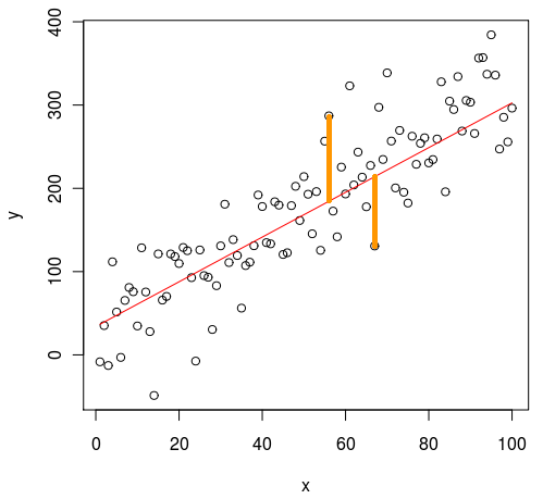
Least squares
Figure showing the direction of the distances minimized by a standard least squares approach. Image taken from Cerebral Mastication blog
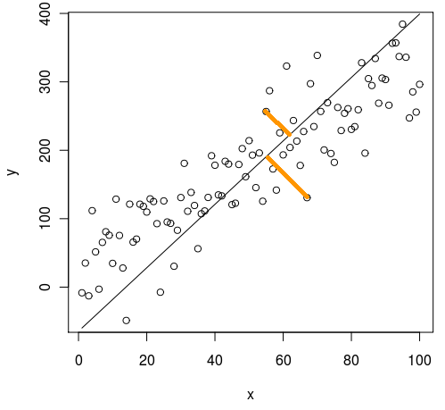
PCA
Figure showing the direction of the distances minimized by a PCA. Image taken from Cerebral Mastication blog
How do I use it?
Preparing the dataThe first step is obviously to take your raw data and transform it in such a way as to maximise the amount of information we can get out of the PCA. In practice this means taking the following steps:
- Convert any text data, such as names or similar, to numerical data. The PCA algorithm does not handle non-numerical data well for obvious reasons.
- Deal with NaN data. For the same reason as above, any datapoints that are NaN either need to be removed or replaced with a suitable number.
- Standardising the data. Since what we are trying to measure is directions of maximal spread in the location of the datapoints it is implicitly assumed that all dimensions 'are created equal' i.e. that they have similar scales and can be compared fairly. Since the units of the variables making up a dataset in general are different this is not the case out-of-the-box. For example, in the data that I am working on we have both Lyman alpha luminosities, which are of the order of 10⁴² and dust extinction, which is of the order of 10⁻¹. It is clear that, unless we rescale our variables somehow, the Lyman alpha luminosity will completely dominate the variance in the sample.
Therefore we standardise the data by subtracting the mean from each variable and 'whiten' the the noise by dividing with the standard deviation:
standardized_var = (var - mean(var)) / std(var)
from sklearn.decomposition import PCA
pca_2c = PCA(n_components=0.95)
pca_res = pca_2c.fit_transform(standardizedData)
# Show how much variance is explained:
print(pca_2c.explained_variance_ratio_.sum())
What are the limitations:
There are a few limitations to the usefulness of this technique. This is by no means a comprehensive list, but simply things I have encountered and feel are relevant to the work I'm doing.- Sensitivity to outliers.
According to this article, and similar sources, PCA is very sensitive to outliers in the data. Intuitively this makes sense since the procedure finds the directions of maximum variance and hence should be dragged significantly by outlying data and scatter in the data set. There are ways to limit this but they appear to significantly increase the complexity of the procedure. - Somewhat difficult interpretation
It is not obvious how the principal components should be interpreted in terms of the physical variables. There are a few of ways that one can try to achieve an interpretation of the PCA results. The first is to write out the form of the PCA components more explicitly to see what the loadings are and examine the linear combination of physical variables explicitly. The second way is to calculate the correlations between the principal component vector and the original data. This will produce a table showing which of the variables are most closely associated with each principal component. The third way, if fitting for instance a plane and is to rewrite the plane back into the 'normal' data coordinate representation.
Useful links and sources:
Cerebral Mastication BlogStack Exchange Question with very good animations
The shape of data blog
Penn State University, online Statistics course
University of Otago, New Zealand, Student tutorial document (pdf)