


Solving the Euler equations analytically is only possible in a few
simple cases. For more general solutions one has to use a numerical
approach. The first step is to discretise space and time:
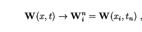 |
(13) |
Solving the Euler equations using normal methods for differential equations is not a good idea. One reason is that the solutions can contain shocks, i.e. very steep gradients, which are not handled well by these methods. Another reason is that the solutions should be conservative, no mass or energy should appear or disappear, and this is generally not guaranteed by these methods. Therefore special methods have been developed to deal with the Euler equations.
Gauss divergence theorem says that for a differential equation
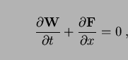 |
(14) |
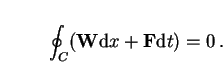 |
(15) |
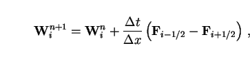 |
(16) |
Once such a way is chosen, it can used for updating the state vector for consecutive timesteps, that way following the evolution of W with time. Choosing the time steps should be done carefully, see section 1.5.2.
For this we use a method called the Roe solver, based on the work of Roe (1981). A description of the ideas behind it (together with a lot of useful background on numerical hydrodynamics) can be found in his review paper from 1986 (ask for copies from me).